Table of Contents

Introduction of Rational Functions:
What are the rational functions?
Limits: Brief Introduction
- Conditions for the existence of the limit of a function:
- Limits at infinity: Vertical and horizontal asymptotes
Holes in the graph:
Graphing rational functions with oblique(slant) asymptotes
Analysing end behaviour of rational functions
Finding x and y intercepts
Transformations of rational functions
Applications of rational functions in real life
Tips and Tricks for graphing rational functions
Conclusion:

Limits and Graphs of Rational Functions

Darshan M.
May 29, 2023

Table of Contents

Introduction of Rational Functions:
What are the rational functions?
Limits: Brief Introduction
- Conditions for the existence of the limit of a function:
- Limits at infinity: Vertical and horizontal asymptotes
Holes in the graph:
Graphing rational functions with oblique(slant) asymptotes
Analysing end behaviour of rational functions
Finding x and y intercepts
Transformations of rational functions
Applications of rational functions in real life
Tips and Tricks for graphing rational functions
Conclusion:

Introduction of Rational Functions:

Have you ever wondered why some graphs seem to have holes in them?
Why do some lines seem to approach a certain value but never quite reach it?

Rational functions are an important topic of Algebra, Precalculus, and AP Precalculus. It is the key to understanding these phenomena and so much more. Imagine a rollercoaster ride where the track twists and turns, climbs and falls, sending riders on a thrilling journey. In a way, the graph of a rational function is like a rollercoaster ride for your mind – it can be just as exhilarating and unpredictable. But don’t let that scare you away! Understanding rational functions is valuable in fields such as engineering, physics, and economics.

In this blog, we will understand the following concepts:

What are the rational functions?
Limits: Brief Introduction
Limits at infinity: Vertical and horizontal asymptotes
Holes in the graph
Graphing rational functions with oblique (slant) asymptotes
Analysing end behaviour of rational functions
Finding x and y intercepts
Transformations of rational functions
Applications of rational functions in real life
Tips and tricks for graphing rational functions
Conclusion

By the end of this blog, you’ll be able to easily decipher the twists and turns of rational functions and ride the rollercoaster.

So buckle up, and let’s dive into the world of graphs of rational functions.

What are the rational functions?

In our earlier classes, we studied rational numbers. Now the question arises what are the rational functions?

This is an important topic in AP Precalculus Unit 1. Rational functions are the ratios of two polynomial functions where the polynomial function as a denominator can’t be zero. The domain of these functions is all real numbers except the numbers, which makes the denominator polynomial expression zero.

For example:

$f(x)=\frac{x^2-4}{x-2}$

is a rational function which is written in the form

$f(x)=\frac {P(x)}{Q(x)}$

where

$P(x)=x^2-4$

and

$Q(x)=x-2$

and the domain of this rational function is

$x\in R-{2}$

since

$f(x)=\frac{x^2-4}{x-2}=\frac{(x+2)(x-2)}{(x-2)}=x+2$

hence f(x) would have a valid output

$\forall x\in R-{2}$

Limits: Brief Introduction

Consider a function f(x) whose value approaches (Let’s say) L as its input x approaches a. Then this statement can be written mathematically as follows:

$\lim_{x\to a}f(x)=L…..(i)$

Don’t get scared after seeing the above notation. It simply says that

“As x approaches a, f(x) approaches L”

Keep in mind that we are not saying

“When x=a, f(x)=L”

This statement is totally different. We don’t even care about the exact f(x) value at x=a. It may or may not be equal to L, but still, in both of the cases (when f(x)=L at x=0 and when

$f(x)\ne L$

at x=0), equation one will be true.

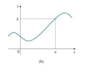
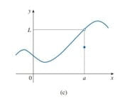
Before you become more confused, let’s get rid of this confusion with the help of three grapes of f(x) shown below-

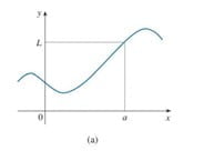
In the first graph you can see f(x)=L at x=a
In the second graph, f(x)= undefined at x=a
In the third graph
$f(x)\lt L$

at x=a

But one thing is common in all these three graphs that is

“As x approaches a from left and right side, f(x) approaches L”

It doesn’t matter what is happening at x=a, but the thing that matters is what does it seem to be happening at x=a. So all three graphs have a common mathematical property that is-

$\lim_{x\to a}f(x)=L$

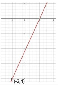
Conditions for the existence of the limit of a function:

The function should approach the same value (output) when X approaches the same value from the left and right sides.

For example:

$\lim_{x\to 0}f(x)$

does not exist for the graph shown below

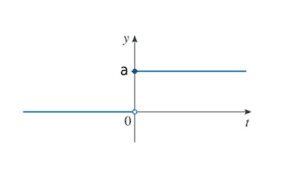
Because as x approaches zero from the left side, f(x) approaches zero, but when x approaches zero from the right side,f(x) approaches a.

So,.

$\lim_{x\to 0^{-}}f(x)\ne \lim_{x\to 0^{+}}f(x)$

Where

$x\to 0^{-}$

says,“As x approaches zero from left side” and

$x\to 0^{+}$

says,“As x approaches zero from the right side “

So, for the existence of limit-

$\lim_{x\to 0^{+}}f(x)=\lim_{x\to 0^{+}}f(x)=L$

as shown in the first three graphs.

2. The function should approach a finite value.

In the graph shown below, as x approaches a, the function approaches infinity. It doesn’t approach a finite single value.

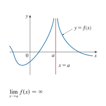
As x becomes closer and closer to a, the function becomes larger and larger.

But in the three figures shown above, as x approaches a, f(x) approaches a finite value L

Limits at infinity: Vertical and horizontal asymptotes

Vertical Asymptote:

Consider a rational function

$f(x)=\frac{1}{x^2}$

Its domain is

$R-{0}$

So we can say that the limit of this function does not exist as x approaches zero. It can be expressed mathematically as follows:

$\lim_{x\to 0}\bigg(\frac{1}{x^2}\bigg)=\infty…..(ii)$

This end behaviour of the function is shown below in the graph.

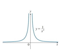
Note: it should not be misinterpreted that the limit of the function exists as x approaches 0.

The only thing equation (ii) tells us is that as x becomes closer and closer to zero, f(x) becomes larger and larger ( tends to positive infinity).

Similarly, we can interpret

$\lim_{x\to 0}\bigg(\frac{1}{x^2}\bigg)=-\infty$

In this case, the vertical line approached by the curve of f(x) (x=0 in this case) is called a vertical Asymptote.

x=a is called the vertical Asymptote of this function if at least one of the following is true-

$\lim_{x\to a^{-}}f(x)=\infty,\lim_{x\to a^{+}}f(x)=\infty,\lim_{x\to a}f(x)=\infty$

$\lim_{x\to a^{-}}f(x)=-\infty,\lim_{x\to a^{+}}f(x)=-\infty,\lim_{x\to a}f(x)=-\infty$

Too difficult to understand? Connect with an AP Precalculus tutor and get personalized help!

Horizontal Asymptote:

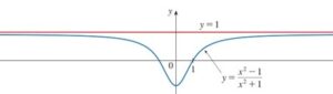
Now consider another rational function that is

$\frac{(x^2-1)}{(x^2+1)}$

its graph is shown below

Divide numerators and denominators by the higher degree of the denominator that is

$x^2$

then

$f(x)=\frac{1-\frac{1}{x^2}}{1+\frac{1}{x^2}}$

When x approaches positive or negative infinity, f(x) approaches 1.

It can be written mathematically as:

$\lim_{x\to -\infty}f(x)=\lim_{x \to +\infty}f(x)=1$

$Or$

$\lim_{x\to -\infty}\bigg(\frac{x^2-1}{x^2+1}\bigg)=\lim_{x \to +\infty}\bigg(\frac{x^2-1}{x^2+1}\bigg)=1$

Note: It should be clear to you that the limit of the function does not exist as

$x \to +\infty$

$x \to -\infty$

because x is not approaching the same input from both left and right side.

We are not saying

$x \to {\infty}^{+}$

$x \to {\infty}^{-}$

but

$x \to -\infty$

$x \to +\infty$

Bonus point: Think about it on your own to understand it in a better way.

In the graph shown above the horizontal line which is approached by the function is called the horizontal Asymptote of the function.

“A horizontal line of equation y=L will be called horizontal Asymptote of a function f(x) when one or both of the following conditions are true-

$\lim_{x\to -\infty}f(x)=L$

$Or$

$\lim_{x\to +\infty}f(x)=L$

Holes in the graph:

A rational function may have a “hole” in its graph in certain cases. A hole occurs when both the numerator and denominator of the function have a common factor that can be cancelled out.

For example, consider the rational function

$f(x) = \frac{(x^2 - 4)}{(x + 2)}$

. At first glance, there may seem to be a vertical asymptote at x = -2, since the denominator approaches zero at that point. However, if we factor in the numerator, we get:

$f(x) = \frac{(x + 2)(x - 2)}{(x + 2)}$

Notice that (x + 2) is a common factor in both the numerator and denominator. We can cancel it out, which gives us:

f(x) = x – 2

Interesting fact: What if we put the original rational function in Desmos? Check it out!

Now, we can see that there is no longer a vertical asymptote at x = -2, since the factor (x + 2) no longer appears in the denominator. Instead, there is a “hole” in the graph at x = -2, since the function is undefined at that point. However, the function approaches the same value from both sides of the hole, which is given by the simplified expression x – 2.

To graph this function, we can plot a point at (2,0), which is where the function has a hole. Then, we can plot other points on either side of the hole and use the simplified expression x – 2 to fill in the gap at the hole. This gives us a smooth, continuous graph of the function that accounts for the hole.

Graphing rational functions with oblique(slant) asymptotes

In addition to horizontal and vertical asymptotes, some rational functions may have oblique asymptotes. An oblique asymptote is a slanted straight line that the graph of a rational function approaches as x goes to positive or negative infinity.

To find the equation of an oblique asymptote, we need to perform a long division between the numerator and denominator of the rational function. The result of the division is a polynomial, which can be used to find the equation of the oblique Asymptote.

For example, consider the function

$f(x) = (x^3 + 2x^2 - 5x + 6)/(x^2 + 1)$

. To find the equation of the oblique Asymptote, we perform long division. The result of the long division is x-2, which is a linear polynomial. Therefore, the equation of the oblique Asymptote is y = x-2.

To verify that this is indeed the equation of the oblique Asymptote, we can graph the function and the Asymptote together:

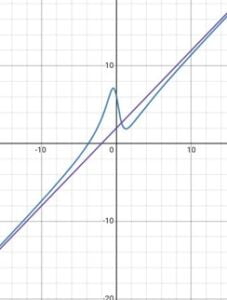
The result of the long division is x-2, which is a linear polynomial. Therefore, the equation of the oblique Asymptote is y = x-2.

To verify that this is indeed the equation of the oblique Asymptote, we can graph the function and the Asymptote together: As we can see from the graph, the function approaches the line y = x-2 as x goes to positive or negative infinity.

Oblique asymptotes can provide us with valuable information about the behaviour of a rational function as x goes to positive or negative infinity. By knowing the equation of the oblique Asymptote, we can predict how the function will behave far away from the origin.

Analysing end behaviour of rational functions

The end behaviour of a rational function refers to how the function behaves as x approaches infinity or negative infinity. This behaviour can help us determine the horizontal asymptotes of the function.

To analyse the end behaviour, we first need to find the degree of the numerator and denominator of the rational function. The degree is the highest power of x in the polynomial.

Case:1 If the degree of the numerator is less than the degree of the denominator, the function approaches zero as x approaches infinity or negative infinity. In this case, the horizontal Asymptote is the x-axis (y=0).

Statement proof:-

$f(x)=\frac{2x+1}{3x^2+4x+1}$

Now we will divide the numerator and denominator by the highest power of x in the denominator that is

$x^2$

, we will get

$f(x)=\frac{\frac{2}{x}+\frac{1}{x^2}}{3+\frac{4}{x}+\frac{1}{x^2}}$

As x will become larger or smaller,

$\frac{1}{x^2}$

term in the numerator will dominate (it means the term

$\frac{1}{x^2}$

will grow faster than another term

$\frac{2}{x}$

so that we can neglect the effect of

$\frac{2}{x}$

in comparison with

$\frac{1}{x^2}$

as x varies) and hence the numerator will approach 0 as x approaches positive or negative infinity.

Similarly

$\frac{1}{x^2}$

term will grow faster in comparison with

$\frac{4}{x}$

$\frac{1}{x^2}$

term will dominate.

As x approaches positive or negative infinity,

$\frac{1}{x^2}$

will approach 0, and the denominator will approach 3.

In the summary, we can say that as

$x\to \infty$

$x\to -\infty; f(x)\to 0$

Case:2 If the degree of the numerator is equal to the degree of the denominator, the function approaches a horizontal line as x approaches infinity or negative infinity. In this case, the horizontal Asymptote is the ratio of the leading coefficients of the numerator and denominator.

Statement proof:- Consider

$f(x)=\frac{2x^3+4x^2-x}{3x^3-5x+1}$

Again, divide the numerator and denominator by the highest degree of the denominator polynomial that is

$x^3$

then

$f(x)=\frac{2+\frac{4}{x}-\frac{1}{x^2}}{3-\frac{5}{x}+\frac{1}{x^2}}$

Again we can say as x approaches positive or negative infinity, the denominator will approach 2 and the numerator will approach 3 then the function will approach

$\frac{2}{3}$

, which is the ratio of leading coefficient of numerator and denominator.

Case:3 If the degree of the numerator is greater than the degree of the denominator, the function approaches positive or negative infinity as x approaches infinity or negative infinity. In this case, there is no horizontal asymptote.

Statement proof:- Consider

$f(x)=\frac{(3x^3+2x^2-5x+1)}{(x^2+1)}$

Now, again divide the numerator and denominator by the highest degree of the denominator polynomial expression which will give us-

$f(x)=\frac{3x+2-\frac{5}{x}+\frac{1}{x^2}}{1+\frac{1}{x^2}}$

Now as x approaches positive infinity or negative infinity, f(x) will also approach positive or negative infinity, depending upon the sign of leading coefficients of numerator and denominator polynomial expression.

Finding x and y intercepts

To fully understand the behaviour of a rational function, it’s important to know how to find its x and y intercepts. The x-intercepts are the points where the graph of the function intersects the x-axis, and the y-intercepts are the points where the graph intersects the y-axis.

To find the x-intercepts of a rational function, we need to solve the equation f(x) = 0. In other words, we need to find the values of x for which the function equals zero. This can be done by setting the numerator equal to zero and solving for x. If the denominator is also zero at any of these values, then those values are not x-intercepts but vertical asymptotes.

For example, consider the rational function

$f(x) =\frac{(x^2 - 4)}{(x - 2)}$

. To find the x-intercepts, we set the numerator equal to zero and solve for x:

$x^2 - 4 = 0$

$(x + 2)(x - 2) = 0$

$x = -2, 2$

So the x-intercepts of the function are at x = -2 and x = 2. Note that x = 2 is not a vertical asymptote since the denominator is not equal to zero at that value.

To find the y-intercept of a rational function, we need to evaluate the function at x = 0. In other words, we need to find the value of y when x equals zero. This can be done by simply plugging in x = 0 into the function and simplifying.

For example, using the same function

$f(x) = \frac{(x^2 - 4)}{(x - 2)}$

, we can find the y intercept by setting x = 0:

$f(0) = \frac{(0^2 - 4)}{(0 - 2)}$

$f(0) = 2$

So the y-intercept of the function is at y = 2. This means that the graph of the function intersects the y-axis at the point (0,2).

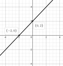
Knowing the x and y intercepts of a rational function can help us sketch its graph accurately and understand its behaviour near the intercepts.

Transformations of rational functions

Transformations of rational functions refer to how we can change a basic rational function’s shape, position, and behaviour by applying certain mathematical operations to it.

The basic rational function is

$f(x) = \frac{1}{x}$

, which has a vertical asymptote at x=0 and a horizontal asymptote at y=0.

To shift this function horizontally or vertically, we can add or subtract values inside or outside the function.

For example, if we want to shift the function to the right by 2 units, we can use the function

$f(x) =\frac{1}{x}-2$

, which will have a vertical asymptote at x=2 instead of x=0.

Similarly, if we want to shift the function upwards by 2 units, we can use the function

$f(x) = \frac{1}{x}+ 2$

, which will have a horizontal asymptote at y=2 instead of y=0.

To stretch or compress the function, we can multiply or divide the numerator or denominator by a constant value.

For example, if we want to stretch the function vertically by a factor of 2, we can use the function

$f(x) = \frac{2}{x}$

, which will have a steeper slope towards the vertical Asymptote.

On the other hand, if we want to compress the function horizontally by a factor of 2, we can use the function

$f(x) = \frac{1}{2x}$

, which will have a shallower slope towards the horizontal Asymptote.

Transformations can also affect the location of the vertical and horizontal asymptotes. Horizontal shifts can affect the location of vertical asymptotes, while vertical shifts can affect the location of horizontal asymptotes. Stretching or compressing the function can change the slopes of the asymptotes, making them steeper or shallower.

Understanding these transformations is important to graph rational functions accurately and efficiently. We can quickly and easily graph various rational functions with different shapes and behaviours by applying the appropriate transformations to the basic function.

Applications of rational functions in real life

Rational functions have a wide range of applications in real-life scenarios.

For example, in economics, rational functions can be used to model cost and profit functions, which can help businesses optimise their production and pricing strategies.

In physics, rational functions are used to model various phenomena, such as fluid flow and oscillations

Rational functions can be used in engineering to model transfer functions in control systems and electrical circuits.

Another application of rational functions is in the field of medicine. The human body has various physiological functions that can be modelled using rational functions.

For instance, a drug’s absorption rate in the bloodstream can be modelled using a rational function.

This information is important for determining patients’ medication dosage and frequency.

Rational functions are also used in the field of finance. They are used to model interest rates, loan payments, and investment growth. By using rational functions, investors can make informed decisions about how to invest their money and how much interest they can expect to earn over a certain period.

In summary, rational functions have a broad range of applications in various fields, including economics, physics, engineering, medicine, and finance. Understanding rational functions is crucial in these fields, as they help to model complex phenomena and make informed decisions.

Tips and Tricks for graphing rational functions

Graphing rational functions can be a challenging task, but there are a few tips and tricks that can make the process easier.

First, it’s important to identify the vertical and horizontal asymptotes of the function. This information can be used to determine the function’s behaviour as it approaches certain values.

Another useful tip is to factor the numerator and denominator of the rational function. This can help to identify any holes in the graph and simplify the function, making it easier to analyse.

Transformations can also be applied to rational functions, just like with other types of functions. These transformations can shift, stretch, or reflect the graph of the function, which can provide valuable information about the behaviour of the function.

Finally, it’s important to remember that practice makes perfect. Graphing rational functions can be challenging at first, but with enough practice, it becomes easier to identify patterns and predict the behaviour of the function.

Conclusion:

In conclusion, graphs of rational functions can be complex and challenging, but they are a powerful tool for modelling real-life phenomena. By understanding the behaviour of rational functions, we can make informed decisions in economics, physics, engineering, medicine, and finance. With the tips and tricks provided in this blog, graphing rational functions becomes easier, and it becomes easy to ride the rollercoaster of rational functions.

Struggling with Quadratic equations as well? Check out Quadratic equations and its Application

About Colin Phillips

Lorem ipsum dolor amet, conse cetur adipisicing elit, sed do eiusmod tempor incididunt labore et dolore

Limits and Graphs of Rational Functions

Introduction of Rational Functions:

What are the rational functions?

Limits: Brief Introduction

Conditions for the existence of the limit of a function:

Limits at infinity: Vertical and horizontal asymptotes

Holes in the graph:

Graphing rational functions with oblique(slant) asymptotes

Analysing end behaviour of rational functions

Finding x and y intercepts

Transformations of rational functions

Applications of rational functions in real life

Tips and Tricks for graphing rational functions

Conclusion:

Share

About Colin Phillips

Quick Links

Services

Others

Contact us

Subjects